ICE CREAM CS 175: Project in AI (in Minecraft) -- Minecraft Biome Landscape Image Completion
Video
Project Summary
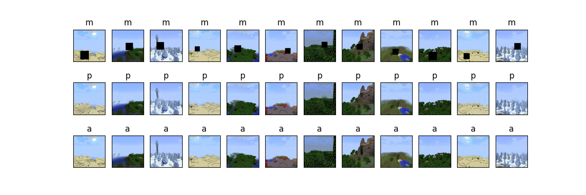
Given masked image ‘m’ our AI will complete ‘m’ to produce reconstructed image ‘p’ so that ‘p’ and the original image ‘a’ are similar
Given masked images of different Minecraft biomes our AI will predict and complete the correct biome. We should be able to complete the image by filling masks of varying, random square size and location. We want the reconstructed images by our AI to be similar to the original unmasked image. Our AI will train on a database of biome images, learning what the features of each complete biome image look like. It will then be able to use this knowledge to finish constructing the masked parts of images that it receives.
Image completion and prediction have useful real world applications. For example, in augmented reality applications, digital items that are placed in the world should look realistic. So when placing a reflective item, that item must reflect parts of the world not in our view. Image prediction can be used to estimate these reflections. Image completion can be used to recreate full faces of people when we only know portions of their face, this ability can be helpful for law enforcement. Image completion can also help us recreate damaged photos with historical or sentimental importance.
Approaches
Data Collection
We gathered our dataset by taking screenshots of various biomes in the Minecraft world (around 10,000 256x256 photos). We created an automated script to complete this task on specific seeds and manually filtered out poor quality photos afterwards. Our training script creates random masks for these photos, which is then used to train our autoencoder.
First Approach
Initially, we attempted to use a GAN model. A GAN is a model made of two neural networks, a generator which generates fake images and a discriminator which classifies the images it receives as real or fake. The goal is to train the generator to fool the discriminator, leading to a model that can generate realistic images. GAN models are generally known to require a large amount of data and training to complete. We experienced this first hand and became blocked due to GPU constraints since our GAN model did not converge. We also had difficulty adapting our GAN, which took input of latent points, to take input of masked images.
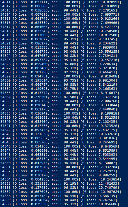
We decided to pivot to an autoencoder model which required less training time and data.
Second Approach
An autoencoder is also composed of two neural networks, an encoder and a decoder. Given an image the encoder compresses the image and the decoder decompresses the encoder’s compressed image to reconstruct the original image. The goal is to have the decompressed image closely resemble the original image with minimal loss. In this way, the autoencoder learns the important features of the images it trains on so that it can effectively compress images with less loss.
This feature learning is particularly useful for our goal of completing masked portions of biomes. For our autoencoder, the encoder consists of a stack of Conv2D and MaxPooling2D layers, while the decoder consists of a stack of Conv2D and UpSampling2D layers.

The encoder’s Conv2D layers are convolutional layers that use 300 filters of kernel size 7x7. Since our images are of size 128x128, filters of size 7x7 seemed to be the right size, not too small or big that we could not identify any features. Filters work in a convolutional layer by looking at a portion of an image by its filter size and shifting the filter by fixed strides over the image until the whole image has been observed. The filters are responsible for identifying and learning the important features of the image. We used a large number of features to better detect features, especially since the masks would add noise during training. These layers use ReLu as an activation function, a popular activation function for image related models.
The encoder’s MaxPooling2D layers are used to reduce overfitting on features learned in the Conv2D layers. These layers pool 2x2 blocks/neurons from the Conv2D layers into 1 neuron based on the maximum value in the 2x2 blocks/neurons. This way, important features are kept and noisy features are ignored before moving onto the next layer.
The decoder’s Conv2D layers are also responsible for feature detection. These layers take the compressed features and identify them for their features. With this feature “mapping”, the identified features can then be decompressed/extracted/upscaled with UpSampling2D layers. This chain of Conv2D and UpSampling2D layers will identify the compressed features and decompress/extract them to an identifiable image. Our decoder uses a sigmoid activation function.
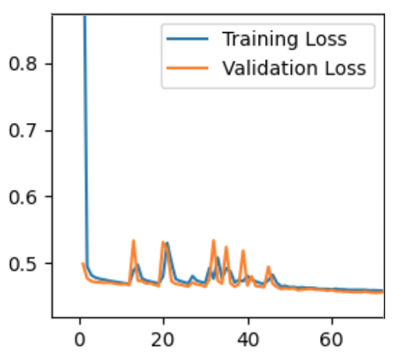
Our autoencoder was trained on 28732 images covering 6 biomes for 70 epochs of batch size 32. While 70 epochs may seem like a small number, each epoch took an average of 20 minutes to complete. We only used a subset of our dataset due to GPU constraints.
Evaluation
Quantitative Results
Our quantitative evaluation is to compare pixel similarity between the autoencoder’s completed image and the original image. We use the loss function of our autoencoder to measure this. Our autoencoder’s loss function is binary cross entropy, which measures whether the pixels are the same or not. So an image’s loss is the average of how many pixels did not match between the completed and original image. Although this is a very strict measure (the human eye can’t tell the difference between pixel colors that are off by 1 or 2), it provided us with enough information to know how our model was doing. A low loss would indicate that most of the pixels were the same, and vice versa. Our model converged at a loss of 0.4536, keep in mind that our loss function was looking at pixels that matched perfectly. Therefore, we also relied on qualitative evaluations.
An alternative loss function would have been to use something like mean squared error (MSE). However, we found that the MSE values tended to get really small, making it hard for us to tell if our model was really making good progress or not.
Qualitative Results
After our model finishes training, it outputs some sample images (in groups of masked image, completed/patched image, and actual/original image). We manually look at these images, and compare them to the original images to see how well completed those images look. Depending on the results, we would go back and tweak our autoencoder, hoping to receive better images. In the end, we still have some blur in the completed images. We found that more filters in combination with a bigger kernel size would result in better quality images. However, due to GPU constraints we were unable to further increase the number of filters used and kernel sizes in our layer.

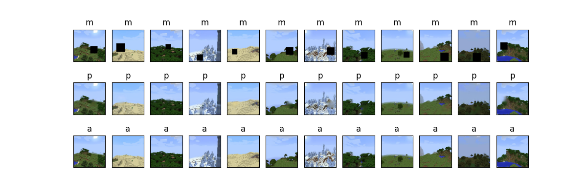
We also have two other qualitative evaluations to collect more qualitative results from our model.
One of the qualitative evaluations has the autoencoder complete on the same image multiple times, but has the mask size increase each time. This allows us to determine the maximum mask size that our AI could currently handle. We tried to increase the size of the mask that our autoencoder could handle by increasing the kernel size in our layers (we saw improvement when we increased kernel size from 5 to 6 to 7), but faced issues with GPU memory (couldn’t increase it past 7).
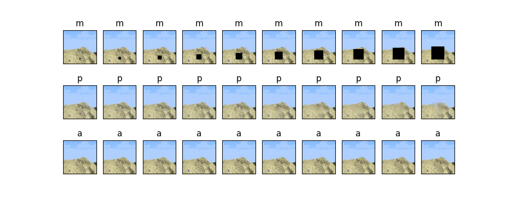
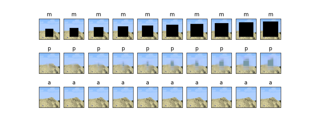
Images are predicted with kernel size 7. Mask size starts as 5x5, increased by 5 every time.
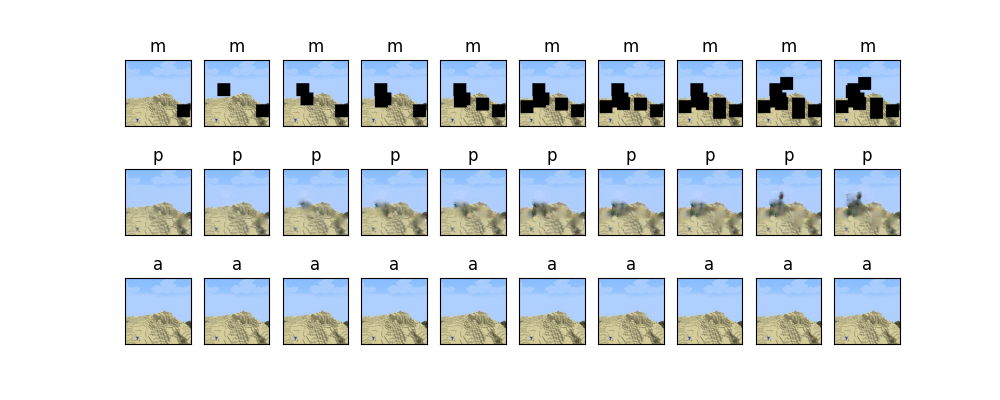
The other qualitative evaluation also has the autoencoder complete on the same image multiple times, but this time the number of masks increases each time. This was more of something interesting that our team wanted to test (seeing how many masks we could put on the same image). We learned that we can add multiple masks and the autocoder will not have problems, but it has problems if the size of the ‘effective mask’ grows in size (for example, masks overlap when placed randomly).
References
https://www.tensorflow.org/tutorials/generative/autoencoder
https://blog.keras.io/building-autoencoders-in-keras.html
https://github.com/jennyzeng/Minecraft-AI/blob/master/src/Data_Collection/MC_world_recording.py
https://towardsdatascience.com/gans-vs-autoencoders-comparison-of-deep-generative-models-985cf15936ea
https://towardsdatascience.com/wtf-is-image-classification-8e78a8235acb